Doppler maps

spotter can be used to model time series spectra of non-uniform stars. In this tutorial we showcase some of these features.

Important

The features shown in this tutotrial are still experimental and not tested against ground truth. Use with care!

A simple spotted surface

We first create a surface with a single circular spot

from spotter import Star
from spotter import core, show
import matplotlib.pyplot as plt

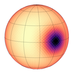
base_star = Star.from_sides(2**4, period=0.02, u=(0.2, 0.2), inc=1.4)
spot = core.soft_spot(base_star.sides, 0.0, 0.0, 0.15)

plt.figure(figsize=(3, 3))
show(base_star - spot, 0.63)

Here we will assume a stellar spectrum made of a single line with a Gaussian profile

import matplotlib.pyplot as plt
import jax.numpy as jnp


def gaussian(x, mu, sigma):
    return jnp.exp(-((x - mu) ** 2) / (2 * sigma**2))


wv = jnp.linspace(400, 410, 500) * 1e-9
star_spectrum = 1 - 0.5 * gaussian(wv, wv.mean(), 0.5e-9)

and we will assume that the star and its spot share the same spectrum.

In spotter, we are in charge of setting the spectrum of each individual pixel. We do that by instantiating the Star object with a spectral spatial map of shape (wavelength, pixels)

import warnings

warnings.filterwarnings("error")

spectra = star_spectrum[:, None] * (base_star - spot).y

star = base_star.set(y=spectra, wv=wv)
star.y.shape

(500, 3072)

This way, star.y holds the len(wv) spatial maps of the star. Here is a plot to realize what that means

from matplotlib import gridspec

idxs = jnp.array([100, 210, 250, 290, 450])

fig = plt.figure(figsize=(7, 3))
axes = gridspec.GridSpec(2, len(idxs))
ax = plt.subplot(axes[1, :])
ax.plot(wv * 1e9, star_spectrum)
ax.plot(wv[idxs] * 1e9, star_spectrum[idxs], ".", c="C0")
ax.set_xlabel("wavelength (nm)")
ax.set_ylabel("normalized flux")
ax.set_title("Stellar spectrum", fontsize=10)

for i, idx in enumerate(idxs):
    ax = plt.subplot(axes[0, i])
    show(star[idx], vmax=1)
    ax.set_title(f"{wv[idx] * 1e9:.1f} nm", fontsize=10)

_ = plt.tight_layout()

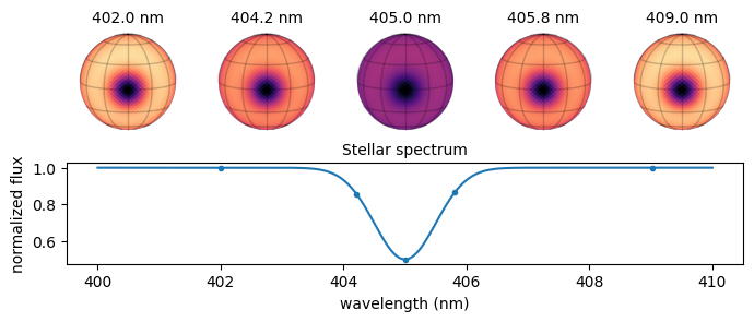
In the last plot we used the fact that star[i] returns the star at the i-th wavelength.

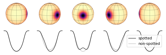
From there we can compute the observed intensity of the star at a given time

from spotter.doppler import spectrum

observed_spectrum = spectrum(star, 0.0)

Let’s plot the observed spectrum at different phases

from spotter.doppler import spectrum

n = 5
fig, axes = plt.subplots(2, n, figsize=(8, 2.5))
nonspotted_spectrum = spectrum(star, star.period / 2)

for i, phase in enumerate(jnp.linspace(jnp.pi / 2, -jnp.pi / 2, n)):
    ax = axes[1, i]
    time = phase * star.period / (2 * jnp.pi)
    ax.plot(spectrum(star, time), c="k", lw=1, label="spotted")
    ax.plot(nonspotted_spectrum, "-", alpha=0.3, c="k", lw=1, label="non-spotted")
    ax.axis("off")

    ax = axes[0, i]
    show(star - spot, phase, ax=ax)

    if i == n - 1:
        plt.legend()

Note

In this example we used the same polynomial limb darkening coefficients across all wavelengths, which is not very realistic. The Star.u argument also accept a set of (wavelength) limb darkening coefficients to be used at each wavelength.

Spectral spatial maps

Because of their cooler temperatures (among other factors), starspots usually have their own spectra, different from the star’s. Hence, in this section, we define the spectra of the star and the spot separately

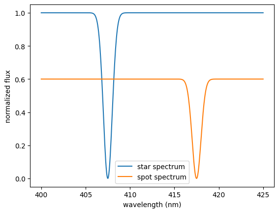
wv = jnp.linspace(400, 425, 500) * 1e-9
star_spectrum = 1 - gaussian(wv, wv.mean() - 0.2 * jnp.ptp(wv), 0.5e-9)
spot_spectrum = 0.6 * (1 - gaussian(wv, wv.mean() + 0.2 * jnp.ptp(wv), 0.5e-9))

plt.plot(wv * 1e9, star_spectrum, label="star spectrum")
plt.plot(wv * 1e9, spot_spectrum, label="spot spectrum")
plt.legend()
plt.xlabel("wavelength (nm)")
_ = plt.ylabel("normalized flux")

The next step consists in setting the spectra of each pixel in the map

import numpy as np

# setting the spectrum of the unspotted part of the star
spectra = (base_star.y - spot) * star_spectrum[:, None]

# setting the spectrum of the spotted part of the star
spectra = spectra + spot[None, :] * spot_spectrum[:, None]
star = base_star.set(y=spectra, wv=wv)

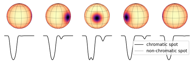
As in the previous example, here is the observed spectrum at different phases

n = 5
fig, axes = plt.subplots(2, n, figsize=(8, 2.5))

for i, phase in enumerate(jnp.linspace(jnp.pi / 1.8, -jnp.pi / 1.8, n)):
    ax = axes[1, i]
    time = phase * star.period / (2 * jnp.pi)
    ax.plot(spectrum(star, time), c="k", lw=1, label="chromatic spot")
    ax.plot(
        spectrum(star, time),
        c="k",
        lw=1,
        alpha=0.3,
        label="non-chromatic spot",
    )
    ax.axis("off")

    ax = axes[0, i]
    show(base_star - spot, phase, ax=ax)

    if i == n - 1:
        plt.legend()