Surface Gaussian Process

In this tutorial we show how to draw a non-uniform surface using a Gaussian Process (GP) on the sphere. Here, we will use this GP to model a star covered in starspots, but of course spotter can be used to model any spherical surface such as that of a planet.

Note

GPs in spotter are defined and computed using the tinygp Python package. For more details about GPs on the sphere, check out the Custom Geometry tinygp tutorial.

The main idea is that a 1D Gaussian Process can be easily defined on the sphere, using the great circle distance as the distance metric in the GP kernel.

Isotropic kernel

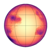
In this first example, we define a kernel to draw a stellar surface uniformly covered with active regions, such as starspots.

We start by defining the properties of our stellar surface with few variables

from spotter import Star

star = Star.from_sides(20, u=(0.4, 0.1))

We can then use tinygp to define an isotropic kernel on the sphere

import tinygp
from spotter.kernels import GreatCircleDistance

kernel = 0.1 * tinygp.kernels.Matern52(0.4, distance=GreatCircleDistance())
gp = tinygp.GaussianProcess(kernel, star.coords)

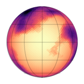
and draw a surface from it

import jax
import matplotlib.pyplot as plt
from spotter import viz

y = gp.sample(jax.random.PRNGKey(4), shape=(1,))[0]
y = 1.0 - y.clip(0.0, 1.0)

plt.figure(figsize=(2, 2))
viz.show(y, u=star.u[0])

Note

Any GP library allowing a custom distance metric can be used in combination with spotter to draw surfaces on the sphere.

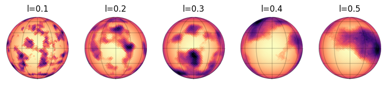
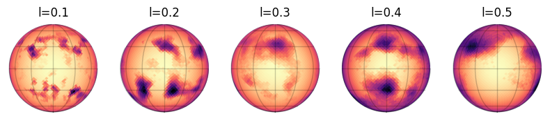
The GP we just built model active regions on a star with sizes related to the kernel length scale. Let’s show surfaces drawn from kernels with different length scales

from matplotlib import gridspec

lenght_scales = [0.1, 0.2, 0.3, 0.4, 0.5]
gridspec.GridSpec(1, 6)
plt.figure(figsize=(12, 2))

for i, l in enumerate(lenght_scales):
    kernel = 0.1 * tinygp.kernels.Matern52(l, distance=GreatCircleDistance())
    gp = tinygp.GaussianProcess(kernel, star.coords)
    y = gp.sample(jax.random.PRNGKey(i + 1), shape=(1,))[0]
    y = 1.0 - y.clip(0.0, 1.0)
    plt.subplot(1, 6, i + 1)
    viz.show(y, u=star.u[0])
    plt.title(f"l={l}")

Active latitudes

As seen on the sun, active regions can be preferentially located at certain latitudes. In order to draw surfaces with such properties, spotter features the ActiveLatitude kernel (non-isotropic!).

This kernel takes an isotropic kernel as input, which sets the active regions properties, as well as their preferred latitude and the standard deviation of the latitude band where they are located.

from spotter import kernels

kernel = kernels.ActiveLatitude(
    kernel=0.1 * tinygp.kernels.Matern52(0.3, distance=kernels.GreatCircleDistance()),
    latitude=0.5,
    sigma=0.2,
    symetric=True,
)

gp = tinygp.GaussianProcess(kernel, star.coords)

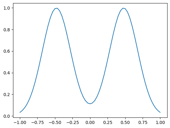
We can plot the distribution of active regions along \(\cos{\theta}\)

import jax.numpy as jnp

cos_theta = star.coords.T[2] / jnp.linalg.norm(star.coords.T, axis=0)
_ = plt.plot(cos_theta, jax.vmap(kernel.amplitude)(star.coords))

and draw a sample from the GP

import jax
import matplotlib.pyplot as plt
from spotter import viz

y = gp.sample(jax.random.PRNGKey(6), shape=(1,))[0]
y = 1.0 - y.clip(0.0, 1.0)

plt.figure(figsize=(2, 2))
viz.show(y, u=star.u[0])

As before, let’s see how surfaces look for different values of the length scale.

from matplotlib import gridspec

lenght_scales = [0.1, 0.2, 0.3, 0.4, 0.5]
gridspec.GridSpec(1, 6)
plt.figure(figsize=(12, 2))

for i, l in enumerate(lenght_scales):
    kernel = kernels.ActiveLatitude(
        kernel=0.1 * tinygp.kernels.Matern52(l, distance=kernels.GreatCircleDistance()),
        latitude=0.5,
        sigma=0.2,
        symetric=True,
    )
    gp = tinygp.GaussianProcess(kernel, star.coords)
    y = gp.sample(jax.random.PRNGKey(i), shape=(1,))[0]
    y = 1.0 - y.clip(0.0, 1.0)
    plt.subplot(1, 6, i + 1)
    viz.show(y, u=star.u[0])
    plt.title(f"l={l}")

We note that the kernel doesn’t have to be symmetric in latitudes.

kernel = kernels.ActiveLatitude(
    kernel=0.1 * tinygp.kernels.Matern52(0.1, distance=kernels.GreatCircleDistance()),
    latitude=jnp.pi / 2,
    sigma=0.2,
    symetric=False,
)
gp = tinygp.GaussianProcess(kernel, star.coords)

y = gp.sample(jax.random.PRNGKey(0), shape=(1,))[0]
y = 1.0 - y.clip(0.0, 1.0)

plt.figure(figsize=(4, 2))
ax = plt.subplot(121)
viz.show(y, inc=0.8, u=star.u[0], ax=ax, vmin=0, vmax=1)
ax.set_title("north pole")

ax = plt.subplot(122)
viz.show(y, inc=jnp.pi / 2 + 0.8, u=star.u[0], ax=ax, vmin=0, vmax=1)
_ = ax.set_title("south pole")